Regression

Regression: Let \(D = \{(X_{i}, Y_{i}) \mid X_{i} \in R^{n}, y_{i} \in R \} \) be some data (experience). Aim: model the relationship between the dependent variable \(Y_{i}\) and independent variables \(X_{i}^{T} = [x_{i,1}, x_{i,2}, …, x_{i,n}]\).

\(x_{i}\) are also called: regressors, exogenous variables, explanatory variables, covariates, input variables, predictor variables, or independent variables.

\(Y_{i}\) is also called: regressand, endogenous variable, response variable, measured variable, criterion variable, or dependent variable.

Linear regression: linear relationship is assumed between \(Y\) and \(X\). Then the linear regression model, or hypothesis which represents the linear relationship between \(X\) and \(Y\) can be formulated as follows:

\[Y = f(X) = \theta_{0} + \sum_{j=1}^{n}(x_{j}\theta_{j})\]

where coefficients \(\theta_{j}\)’s called unknown parameters, or model parameters. These parameters are often arranged in a vector and we denote it as \(\Theta = [\theta_{0},\theta_{1},\theta_{2},…,\theta_{n}]^{T}\).

Therefore, in this model, the regressand (\(Y\)) is a linear combination of the regressors (\(x_{j}\)).

In other words: the regressand (\(Y\)) is a weighted sum of the input features (\(x_{j}\)).

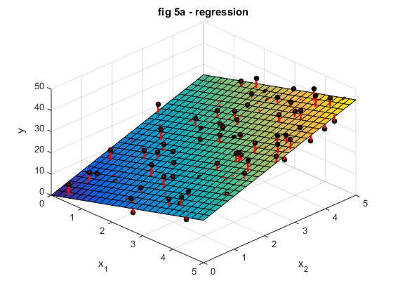
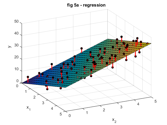
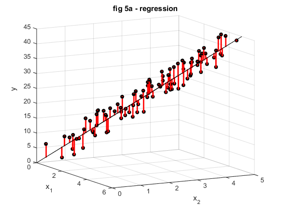
Figure 1. Example of linear regression. Each plot shows exactly the same data but only from different point of views. Data was generated by \(\Theta = [0,5,4]\), with a uniformly distributed error. (\(\theta = 0\) is the bias).

So, what we want is to calculate the model parameter \(\Theta\) somehow. This process is called “learning”.

Regression and Ordinary Least Squares method (OLS):

Typically, having some data (experience) \(D = \{(X_{i},Y_{i})\mid X_{i} \in R^{n}, y_{i} \in R\}\), it is possible to define a performance estimation on how well the parameters \(\Theta\) model the relationship between the dependent and the outcome variables. This performance measure is often called loss function. The most common measure (in this field) is the least squares (L2) defined formally as: \[ J_{1}(\Theta\mid D) = \sum_{i=1}^{m}(Y_{i} - f(X_{i}))^{2} = \sum_{i=1}^{m}\bigg(Y_{i} - \theta_{0} - \sum_{j=1}^{n} x_{i,j}\theta_{j}\bigg)^{2} \]

Many other performance measures could be defined easily for any problem specific tasks. However, the reason why this method has become so popular is perhaps that it makes the loss function \(J\) a convex function with respect to parameters \(\Theta\). (The reason is not that, this loss function is reasonable.) This provides several numerical advantages. Note that, in practice other loss function might be more reasonable, but can make the optimization more difficult. See Figure 2 below.

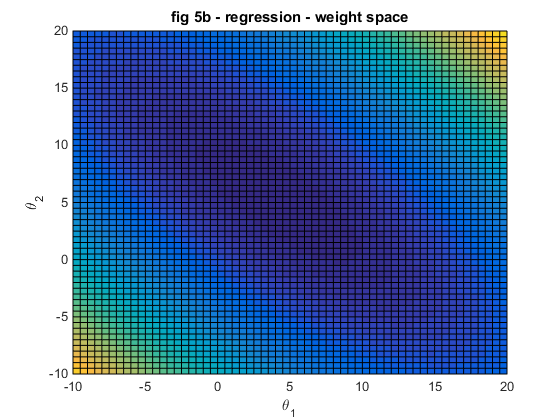
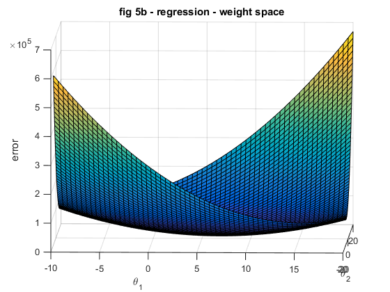
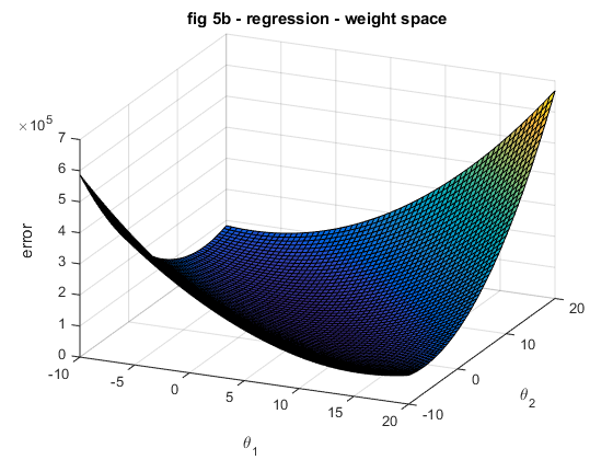
Figure 2. The shape of the error function \(J\) w.r.t \(D\). Each plot shows exactly the same error function from different point of view, obtained from data shown in Figure 1. All three figures show the same function, but from different angle. \(\theta_{0} = 0\) was used.

Regularized regression (ridge regression): It imposes a penalty on the parameter values \(\Theta\).

\[J(\Theta\mid D) = J_{1}(\Theta\mid D) + \lambda\sum_{j=1}^{n}\theta_{j}^{2}\]

The second term is called the regularization term, or penalty term. Here \(\lambda\) is a trade-off parameter that balances between the importance of regularization term and the fitting/cost error. The larger the amount of \(\lambda\) the greater the importance of the regularization, and vice versa. The parameters shrink toward zero and (to each other) when \(\lambda\) increases. Notice that \(\theta_{0}\) (the bias) is not included in the regularization term. The problem to find the \(\widetilde{\Theta}\), which minimizes the error can be formulated as follows:

\[\widetilde{\Theta} = argmin_{\Theta}J(\Theta\mid D) = argmin_{\Theta}\Bigg\{\sum_{i=1}^{m}\bigg(\theta_{0} + \sum_{j=1}^{n}x_{i,j}\theta_{j} - Y_{i}\bigg)^{2} + \lambda\sum_{j=1}^{n} \theta_{j}^{2} \Bigg\} \]

Now, let’s take step back for a moment and take a look at the two formulas (\(F(x)\) and \(J(\Theta\mid D)\)). In the first one, a data \(x\) is a variable and the parameters \(\theta_{i}\) are constants. In the cost functions the data \(x_{i}\) becomes a constant and the model parameters are the variables. In fact, the optimal model parameters are some sort of combination of the data, or at least the optimal solution mostly depends on the data.

This error function is convex w.r.t. \(\Theta\), see an example on Figure 3.

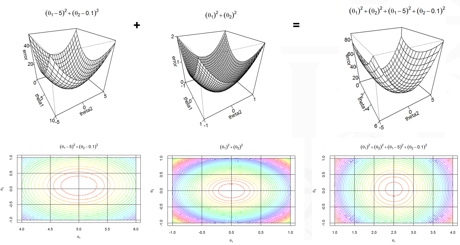
Figure 3. The shape of the regularized error function \(J\) w.r.t. \(D\) The first subplot corresponds to the error term, the second to the regularization term, and the last is the sum of the error and the regularization terms. Note that, the error function is different from the previous examples shown in Figures 4-5.

Solving fitting problems

Normal equations:

Let’s arrange our data \(x\)’s in a matrix from. First, add a constant value 1 to each data: \( X = \left[\begin{array}{cccc} 1 & X_{1} \cr 1 & X_{2} \cr 1 & X_{3} \cr . & . \cr 1 & X_{m} \end{array}\right] = \left[\begin{array}{cccc} 1 & X_{1,1} & X_{1,2} & … & X_{1,n} \cr 1 & X_{2,1} & X_{2,2} & … & X_{2,n} \cr 1 & X_{3,1} & X_{3,2} & … & X_{3,n} \cr & & … & & \cr 1 & X_{m,1} & X_{m,2} & … & X_{m,n} \end{array}\right] \) and let \( Y = \left[\begin{array}{cccc} Y_{1} \cr Y_{2} \cr Y_{3} \cr … \cr Y_{m} \end{array}\right] \)

Then we want the \(\Theta\), which minimizes the least squares error of the following normal equations: \[(X^{T}X + \lambda I)\Theta = X^{T}Y \] We can rearrange the variables and give a closed form for \(\Theta\): \[\Theta = (X^{T}X + \lambda I)^{-1}X^{T}Y \] This solution involves matrix inversion which requires \(O(n^{3})\) time.

Gradient descent algorithm.

This method iteratively approaches an optima of functions. In each cycle it determines the tangent of the function in the current position in order to determine the direction of the optima.

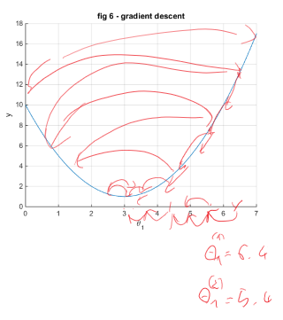
Algorithm 1.

\[ \begin{array}{ll} \text{initialize } \theta_{j} \text{ with random values.} \cr \text{repeat until convergence \{} \cr \hspace{1cm}\widetilde{\theta_{j}} = \theta_{j} - \mu \frac{\partial}{\partial\theta_{j}}J(\Theta\mid D) & \text{for all j ;} \cr \hspace{1cm} \theta_{j} = \widetilde{\theta_{j}} & \text{for all j;} \cr \text{\}} \end{array}
\] Note: update \(\theta_{j}\)’ simultaneously.

The same as above, but in vector form: \[ \begin{array}{ll} \text{repeat until convergence \{} \cr \hspace{1cm}\Theta^{(k+1)} = \Theta^{(k)} - \mu \nabla J(\Theta^{(k)}\mid D) \cr \text{\}} \end{array}
\]

Here: \[ \begin{array}{ll} \frac{\partial}{\partial\theta_{j}}J(\Theta\mid D) = \frac{\partial}{\partial\theta_{j}}(\frac{1}{2m}\sum_{i=1}^{m}(\theta_{0} + \sum_{j=1}^{n}x_{i,j}\theta_{j} - Y_{i})^{2} + \lambda\sum_{j=1}^{n}\theta_{j}^{2}) = \frac{1}{m}\sum_{i=1}^{m}(\theta_{0} + \sum_{j=1}^{n}x_{i,j}\theta_{j} - Y_{i})x_{i,j} + 2\lambda\theta_{j} & \text{for j > 0} \cr \frac{\partial}{\partial\theta_{0}}J(\Theta\mid D) = \frac{\partial}{\partial\theta_{0}}(\frac{1}{2m}\sum_{i=1}^{m}(\theta_{0} + \sum_{j=1}^{n}x_{i,j}\theta_{j} - Y_{i})^{2} + \lambda\sum_{j=1}^{n}\theta_{j}^{2}) = \frac{1}{m}\sum_{i=1}^{m}(\theta_{0} + \sum_{j=1}^{n}x_{i,j}\theta_{j} - Y_{i}) & \text{for j = 0} \end{array} \]

This update rule is called LMS (Least mean squares) update rule, or Widrow-Hoff learning rule.

The parameter \(\mu\) is the learning rate, it controls the size of the step in each iteration. Some technical issues:

1. When \(\mu\) is too small then the convergence becomes slow.
2. If \(\mu\) is too large, then divergence.
3. The magnitude of the update is proportional to the error term: \((Y_{i} - \theta_{0} - \sum_{j}^{n}x_{\{x,j\}}\theta_{j})\)
4. Feature normalization: the range of the feature values needs to be transformed to the same scale

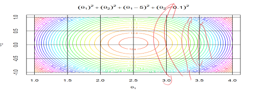
Figure 4. An example of the convergence of the Gradient Descent algorithm when data is not normalized. It converges slowly along with the large scale features and diverges on the small scale features.

There are two common approaches, a) normalization and b) scaling:

a) Normalization consists of two steps:

1. centralization: \(\widehat{x_{i,j}} = x_{i,j} - \frac{1}{m}\sum_{l}x_{l,j} \)
2. standardization: \(\widetilde{x_{i,j}} = \frac{\widehat{x_{i,j}}}{\frac{1}{m}\sum_{l}\widehat{x_{l,j}}^{2}}\)

b) Scaling feature values to the range [0,1], (other ranges work well too, such as, [-1,1], [-3,3], etc.). \(\widetilde{x_{i,j}} = \frac{X_{i,j} - X_{min,j}}{X_{max,j} - X_{min,j}}\)

Batch mode:

In the case above the gradient descent algorithm uses the whole dataset. You can use less data in each iteration, say, you can chose randomly 1, 5, 10, … in each iteration, and calculate the \(\Theta\)’s. This can be often useful if you have lot’s of data, or data access is expensive (over network, etc.) We can repeatedly run through the training set, and each time we encounter a training example, we update the parameters according to the gradient of the error with respect to that single training example only. This algorithm is called stochastic gradient descent (also incremental gradient descent). It slows the convergence down, but uses less data and hence less memory in each iteration.

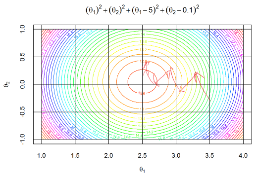
Figure 8. An example path of the stochastic gradient algorithm.

Other optimization methods:

Other optimization methods can be used instead of Gradient Descent, such as:

• Newton’s method,
• Conjugate gradient
• BFGS (Broyden-Fletcher-Goldfarb-Shanno)
• L-BFGS (Limited memory - BFGS)

Each method would take the same input and provide (more-or-less) the same optimum at the output.

Discussion 1. Data comes from some clinical experiment, where 1000 (or 10,000) patients examined and for each patient you have 100,000 features. You need to explore a linear relationship in the data. Which method would you use: 1) Normal equations, or 2) Gradient Descent Optimization. Why?

Discussion 2. Data comes from used car retail shop, where cars are described by 54 features and there are 10,000,000 of such data objects. You need to explore a linear relationship in the data. Which method would you use: 1) Normal equations, or 2) Gradient Descent Optimization. Why?

Comaprison of the Normal Equation method vs. Gradient Descent Optimization.

Both methods aims at finding the same solution, but these two are different in some certain computational aspects.

1. Normal Equation method:
   • (-) \(O(n^{3})\) can be very slow for large number of features.
   • (-) Involves matrix inversion and can be a problem when the matrix becomes singular.
   • (+) Not iterative, and thus does not require leraning rate and termination condition to be specified in advance.
2. Gradient Descent Optimization:
   • (-) It is an iterative method and requires to specify the termination condition advance.
   • (-) Requires the specification of the learning rate parameter.
   • (+) Easy to scale up for paralell computations, better for big data.
   • (-) Requires feature scaling.
   • (+) Easy to extend to other types of loss functions, i.e. this is a more general method, it works with non-convex loss functions as well.

Problems with linear regression in general:

A) Noise, B) non-lienar relationship, C-D) outliers, (Image source: Wikipedia. Anscombe’s quartet)

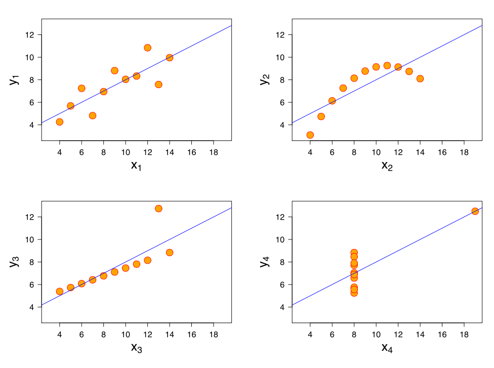
Note that: L2 loss function is very sensitive to outliers. Because it is a quadratic loss. If the error is 1: \(\mid \hat{y} - y \mid = 1\), then the loss adds +1. If the error is \(\mid \hat{y} - y \mid = 10\) , then the loss adds 100, thus the optimizer tries to reduce this error at the expense of increasing the bias of the rest of the data.

E) Simpson’s paradox (Simpson’s paradox is the effect in subgroups of data which disappers or reverses when subgroups are combined)

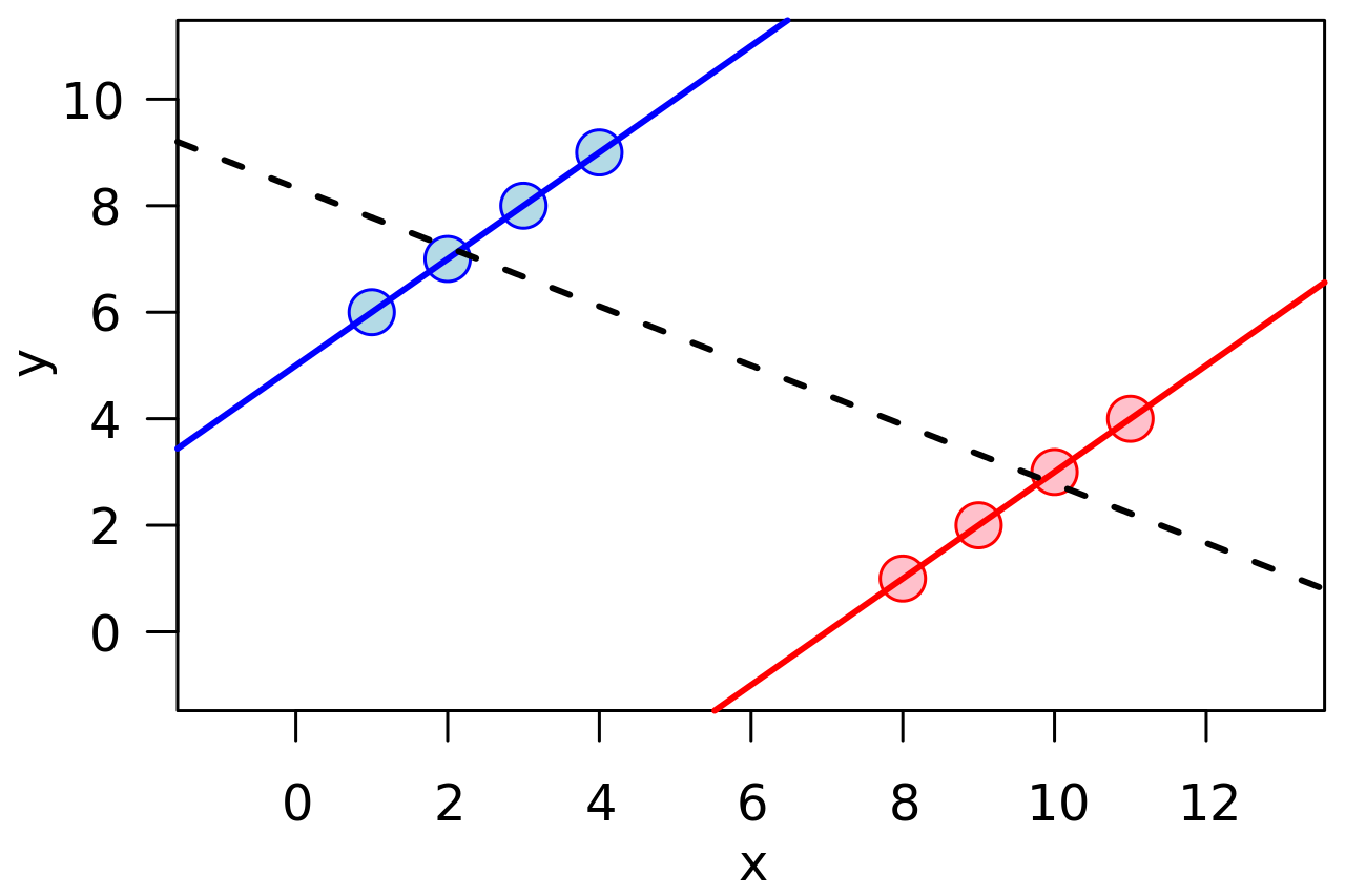
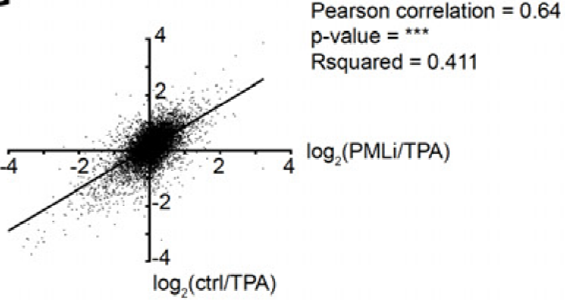
F) An example for (mis-) modelling linear relationship in microarray data. (Source: Lusic et al. Cell Host Microbe. 2013 Jun 12;13(6):665-77, supplementary materials.)

Discussion 3: How would you check that the data fit linearly to the linear model. I.e. how can you check you are not dealing with case B?