LSTM

The RNNs unrolled in time can be represented as follows:

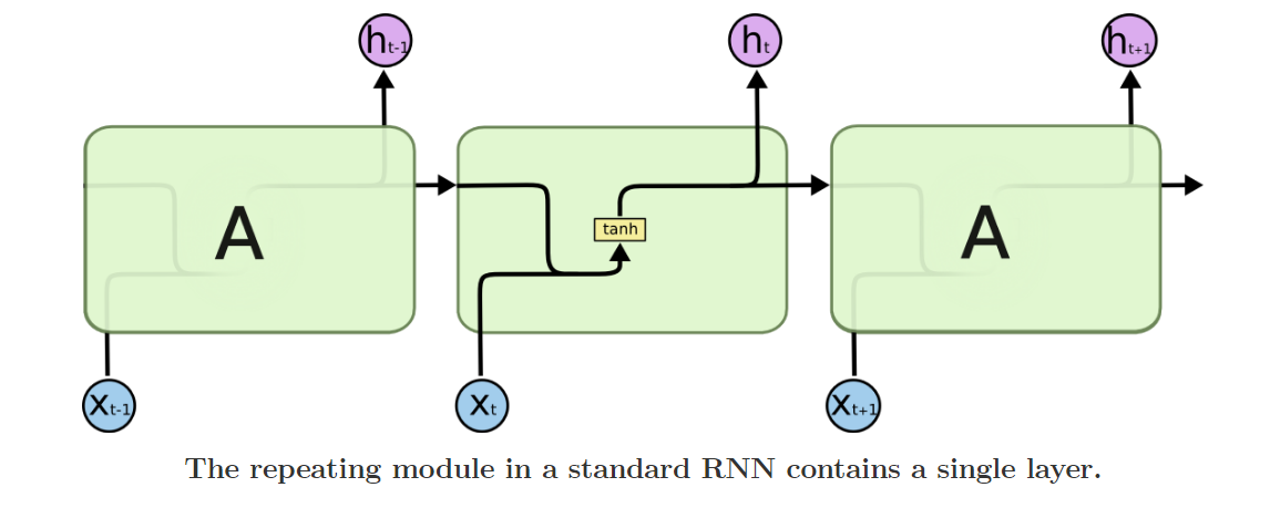
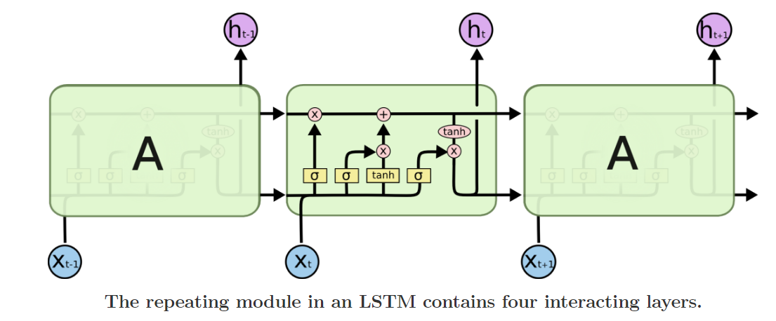
The long-short term memory (LSTM) is also somewhat like this, but it has a more complicated memory update mechanism. LSTMs use a memory and a state. This was done in order to make the model capable of learning long-term dependencies. The core idea of the LSTMs is the state which runs through the whole time. The state is denoted by \(C\) here. An LSTM performs four steps on its state using so called gates. The gates are: input modulation, input gate, forget gate and output gate. The main idea in LSTMs is that each gate is differentiable so their operation can be learned from data.

Let the data be \(x = x_{1}, …, x_{T}\), where each \(x_{i} \in R^{n}\) are column vectors, and the desired outputs are \(y = y_{1}, …, y_{T}\). Let the state vector be \(c \in R^{k}\) and the hidden unit \(h \in R^{l}\). Before, we discuss the operations, let us take a look at the structure of the cell.

The forget gate:

It will calculate which information should be removed from the state \(c\), based on the the input from the previous hidden unit \(h_{t-1}\) and the current input \(x_{t}\). These vectors are combined and transofmed as follows: \[f_{t} = \sigma(W_{f}[h_{t-1};x_{t}] + b_{f})\] where \(\sigma\) is the sigmoid function applied element-wise, \(W_{f} \in R^{x \times (l+n)}, f_{t} \in R^{k}\), and \([,;,]\) denotes vector concatenation.

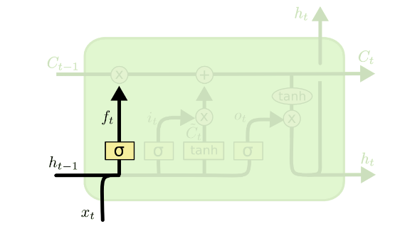
This \(\sigma\) function maps the input \(x_{t}\) and the memory state \(h_{t-1}\) (dim:\(l + n\)) to the state space (dim:\(k\)). The output \(f_{t}\) can be considered as a bit vector, which indicates the components of the state vector \(c_{t}\) to be forgetten. \(f_{t_{i}} \approx 1\) indicates that the \(i\)-th compnent will be kept and \(f_{t_{i}} \approx 0\) indicates the component will be forgotten.

State update gate:

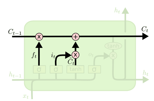
In this step we calculate what information is to be add to the state \(c_{t}\). This step has two parts. First, it calculates a new candidate state vector: \(\widetilde{c_{t}} = tanh(W_{c}[h_{t-1}, x_{t}] + b_{c})\), where \(W_{c} \in R^{k \times (l+n)}\), and \(\widetilde{c_{t}}, b_{c} \in R^{k}\), and then it calculates which information will be updated: \(i_{t} = \sigma(W_{i}[h_{t-1},x_{t}] + b_{i})\), where \(W_{i} \in R^{k \times (l+n)}\), and \(i_{t} \in R^{k}\).

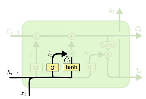
Then, the state vector is updated as follows: \[c_{t} = c_{t-1}\hspace{1mm} ^{\circ} f_{t} + \widetilde{c_{t}}^{\circ} i_{t}\]

where \(^{\circ}\) denotes the element-wise vector multiplication. This step is shown below.

Now, the hidden unit ht is being updated. This step is based on the new state vector. First, it calculates the component indices which should go to the output. These indices will determine which state vector components c_t should go to the output. \[o_{t} = \sigma(W_{0}[h_{t-1},x_{t}] + b_{0})\]

The new memory (hidden state) will be the cell state squased to [-1, +1] using tanh elementwise multiplied with \(o_{t}\). \[h_{t} = o_{t}\hspace{1mm}^{\circ} tanh(c_{t})\]

The emission produced by LSTM may contain additional calculations as well if it is needed: \[y_{t} = softmax(W_{y}h_{t} + b_{y})\]

Now the question is how can we calculate the weight parameters: \(W_{f}, W_{o}, W_{y}, W_{c}, W_{i}\) and the corresponding biases. All steps, sigmoids and tanhs are derivable; thus the calulation can be done easily using the chain rule but is technical. [ref: LSTM: http://colah.github.io/posts/2015-08-Understanding-LSTMs/]

The LSTM’s hidden state is the concatenation \([h_{t};c_{t}]\). Thus, the LSTM has two kinds of hidden states: a “slow” state \(c_{t}\) that fights the vanishing gradient problem and it can be considered as a long-term memory, and a “fast” state \(h_{t}\) that allows the LSTM to make complex decisions over short periods of time. It is notable that an LSTM with n memory cells has a hidden state of dimension \(2n\).

Recall that RNNs easily learn the short-term but not the long-term dependencies. The LSTM addresses the vanishing gradient problem differently.

In the discussion that follows, let \(c_{t}\) denote a hidden state of an unspecified RNN architecture. The LSTM’s main idea is that, instead of computing \(c_{t}\) from \(c_{t-1}\) directly with a matrix-vector product followed by a nonlinearity, the LSTM directly computes \(\Delta c_{t}\) which is then added to \(c_{t-1}\) to obtain \(c_{t}\). At first glance, this difference may appear insignificant since we obtain the same \(c_{t}\) in both cases. And it is true that computing \(\Delta c_{t}\) and adding it to \(c_{t-1}\) does not result in a more powerful model. However, the gradients of an RNN that computes \(\Delta c_{t}\) are nicer as well, since they cannot vanish. More concretely, suppose that we run our architecture for 1000 time steps to compute \(c_{1000}\), and suppose that we wish to classify the entire sequence into two classes using \(c_{1000}\). Given that \(c_{1000} = \sum_{t=1}^{1000} \Delta c_{t}\) (including \(\Delta c_{1}\)) will receive a sizeable contribution from the gradient at timestep 1000. This immediately implies that the gradient of the long-term dependencies cannot vanish. It may become “smeared”, but it will never be negligibly small. [ref: http://proceedings.mlr.press/v37/jozefowicz15.pdf]

Variants of LSTMs:

There are different type of LSTMs, one can build its own structure or modify the one above. The point is that the gates can be used to control the information flow. Certainly, LSTM can be organized into multi-layer network yielding deep LSTMs.

Another approach is that one could combine the update and the forget steps, so the decision on what information to forget and what new information to add could be made simultaneously. This can be done in the following way:

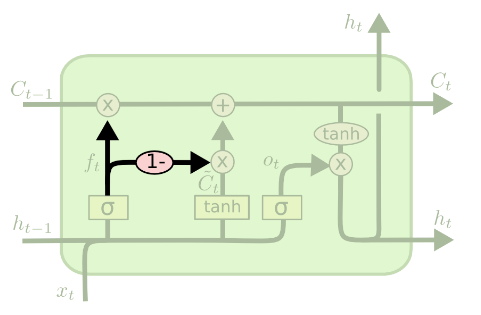
\[c_{t} = f_{t}\hspace{1mm}^{\circ} c_{t-1} + (1 - f_{t})\hspace{1mm}^{\circ}\widetilde{c_{t}}\]

Another variant of LSTM contain peepholes for the gates, so they can incorporate the current state vector into their decisions.

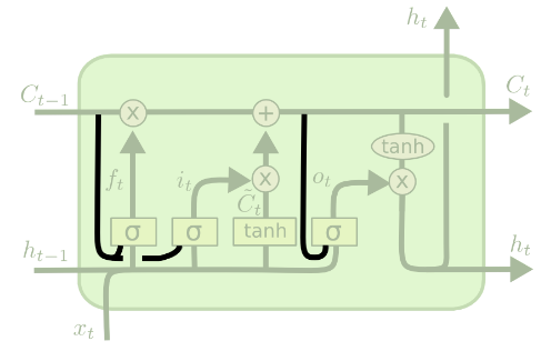
\[f_{t} = \sigma(W_{f}[h_{t-1};c_{t-1};x_{t}] + b_{f})\] \[i_{t} = \sigma(W_{i}[h_{t-1};c_{t-1};x_{t}] + b_{i})\] \[o_{t} = \sigma(W_{0}[h_{t-1};c_{t-1};x_{t}] + b_{0})\]

Another popular variant is the Gated Recurrent Unit (GRU): This method does not use state vector \(c_{t}\), but only the hidden memory vector \(h\) and it also combines the forget and input gates. The resulting model is simpler than a vanilla LSTM because GTU uses only two gates and only one state vector. The first gate is the reset gate: \[r_{t} = \sigma(W_{r}[h_{t-1};x_{t}] + b_{r})\]

\[\widetilde{h_{t}} = tanh(W_{h}[r_{t}\hspace{1mm}^{\circ} h_{t-1},x_{t}])\] In this formulation, when the reset gate is close to 0, then the hidden state is forced to ignore the previous hidden state and reset with the current input.

The second gate is the update gate: \[z_{t} = \sigma(W_{z}[h_{t-1};x_{t}] + b_{z})\]

Finally, the hidden unit is updated as: \[h_{t} = z_{t}\hspace{1mm}^{\circ} h_{t-1} + (1 - z_{t})\hspace{1mm}^{\circ}\widetilde{h_{t}}\] The update gate controls how much information from the previous hidden stat will carry over to the current hidden state. This acts similarly to the memory cell in the LSTM and helps the RNN remember long-term information. [Ref: GRU: https://arxiv.org/pdf/1406.1078v3.pdf]