Adversarial Attack

The aim of adversarial attack (AA) is to create an adversarial example which fully confuses a classifier program. An adversarial example is a sample of input data which has been modified very slightly in a way that is intended to cause a machine learning classifier to misclassify it.

The types of AAs:

• Generate a noise-like data which is confidently labelled by a classifier.
• Generate a real-like picture what is classified with a wrong label with high confidence. In this case, these modifications can be so subtle that a human observer does not even notice the modification at all, yet the classifier still makes a mistake confidently.

Adversarial examples pose security concerns because they could be used to perform an attack on machine learning systems, even if the adversary has no access to the underlying model.

There are two types of AA: white-box model and black-box model. In the case of the white-box model the attacker has an access to the target model and to its derivatives. In the black-box scenario the attacker does not have this access.

1. Generation of real-like adversarial examples.

1.1 White box models.

The attacker has an access to the target model. Let us consider a model, possibly a deep neural network represented by \(f\), input image: \(x\) (a tensor, height, width, and color channels), \(f_{i}(x)\) denotes the confidence (probability) of the classifier that input \(x\) belongs to the \(i\)th class. \(y_{true}\) denotes the true class label of \(x\). Let \(J\) be the usual cost function (cross entropy, etc).

1.1.1 The Fast Gradient Sign method

(by Goodfellow et al: Explaining and harnessing adversarial examples, 2015) proposed the following simple method: \[x^{\ast} = x + \epsilon \cdot sign(\nabla_{x} J(x, y_{true}))\] Note that, the gradients are calculated with respect to the input and not the model parameters. This can be simply done by backpropagation, when the units in first (input) layer is also considered as variables, and simply the derivatives are calculated. Note also that the derivatives are added to the input \(x\), and not substracted like in the case of parameter update. The method above can be written in a different form: \[x^{\ast} = x - \epsilon \cdot sign(\nabla_{x} J(x, y_{fool}))\]

The \(sign(.)\) function basically erases the gradient length (but keeps the direction), and rescales them by \(\epsilon\). The \(y_{fool}\) denotes the incorrect class label we want to obtain for the image \(x^{\ast}\).

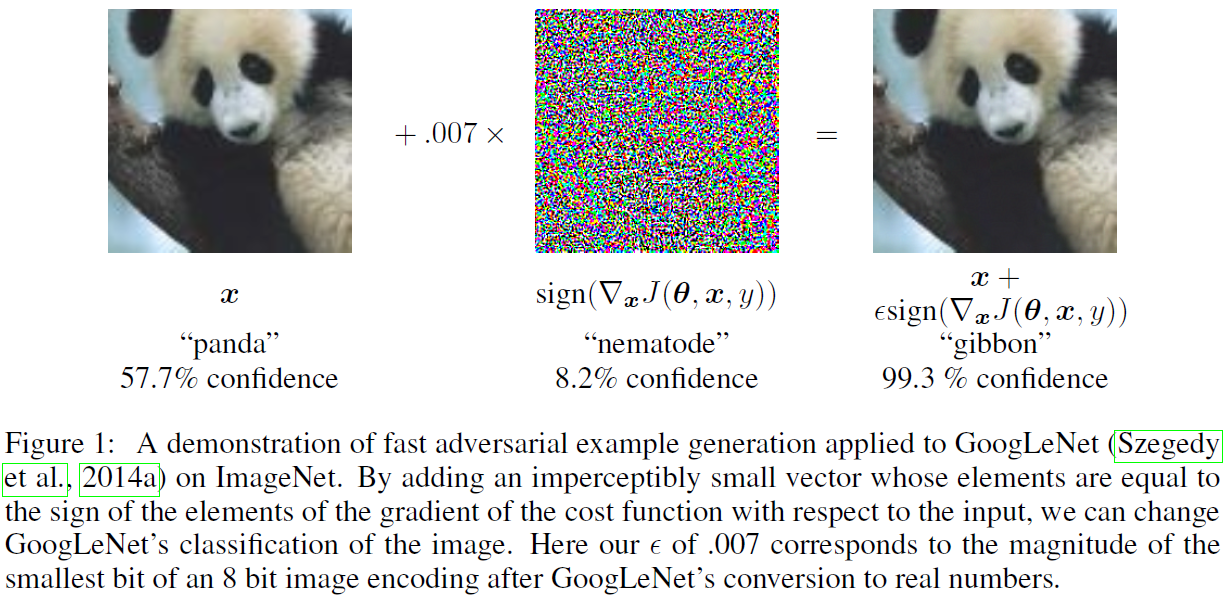
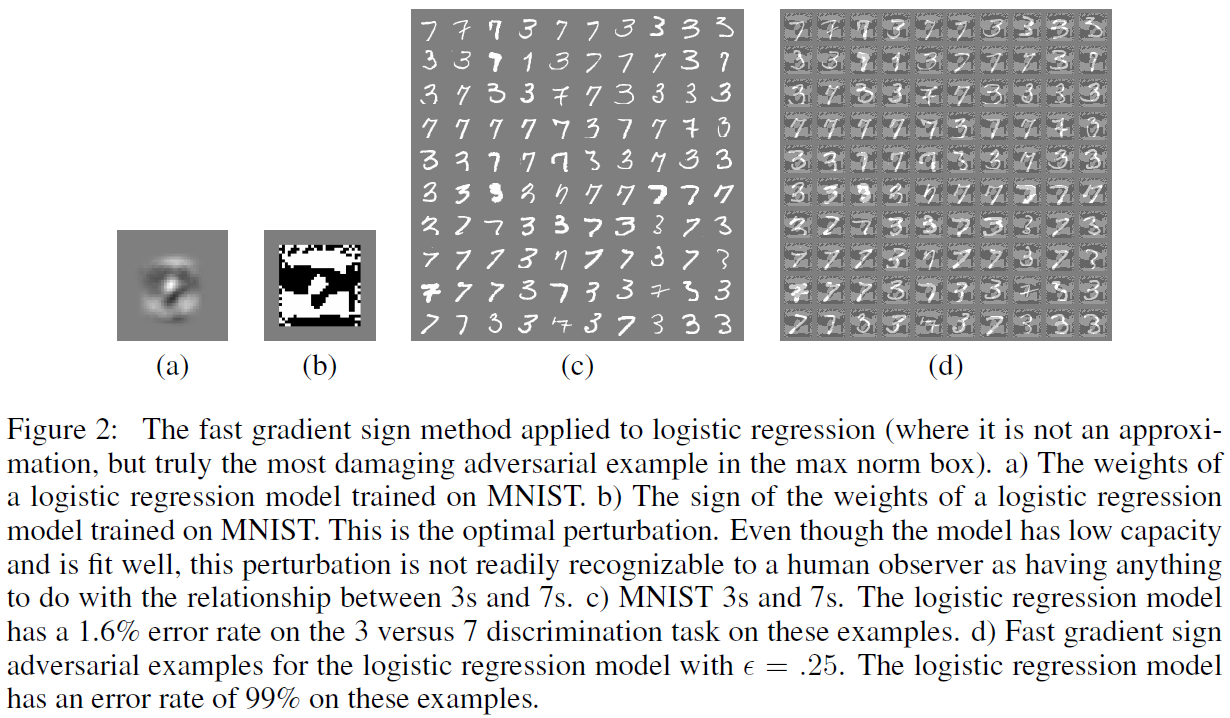
The cause of these adversarial examples was a mystery, and speculative explanations have suggested it is due to extreme nonlinearity of deep neural networks, perhaps combined with insufficient model averaging and insufficient regularization of the purely supervised learning problem. Linear behavior in high-dimensional spaces is sufficient to cause adversarial examples

In image recognition, neural networks are mainly built of linear blocks such as Rectified Linear Unit and Convolutional layers. When such neural network has really lots of parameters, making a little change \(\epsilon\) in each component of an input vector can result in a big change in the output as much as \(\epsilon\lVert W \rVert\). Adversarial training discourages this highly sensitive locally linear behavior by encouraging the network to be locally consistent in the neighbourhood of the training data. This can be seen as a regularization method.

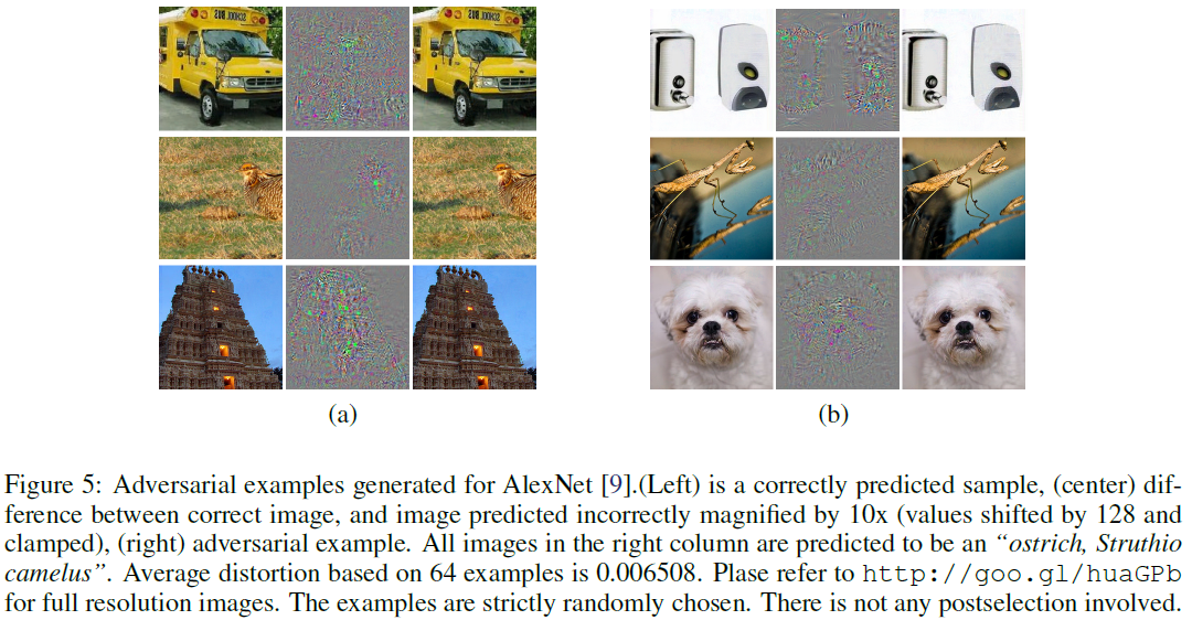
1.1.2 The first approach

to generate adversarial examples was developed by Szegedy et al. [Intriguing properties of neural networks, 2014]. It is an iterative-based method to find a good perturbation \(r\) to fool the classifier: \[min_{r}c|r| + J(x + r, y_{fool})\] subject to \((x + r) \in [0,1]^{m}\),

where \(m\) denotes the dimension of the imput image. The variables to be optimized are in \(r\). This optimizaiton was solved using L-BFGS optimizers.

1.1.3 Adversarial Patches

(developed by Tom Brown: Adversarial Patch, NIPS, 2017) method aims at creating adversarial image patches which can be printed, added to any scene, photographed, and presented to image classifiers; even when the patches are small, they cause the classifiers to ignore the other items in the scene and report a chosen target class.

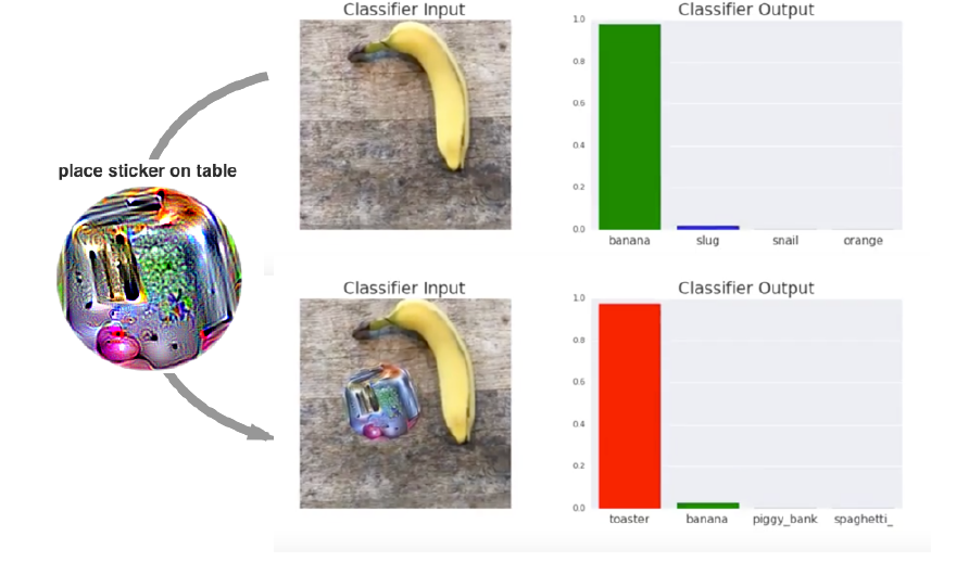
https://youtu.be/i1sp4X57TL4 The training of such patches is a bit technical because we don’t generate a full image but just a small image patch placed on the top of another image. Thus rotation, translation, and scaling operators are involved. Further details can be found in

1. Anish Athalye, Synthesising robust adversarial examples, ICLR, 2018
2. Tom Brown: Adversarial Patch, NIPS, 2017

1.1.4 Adversarial examples as regularizers

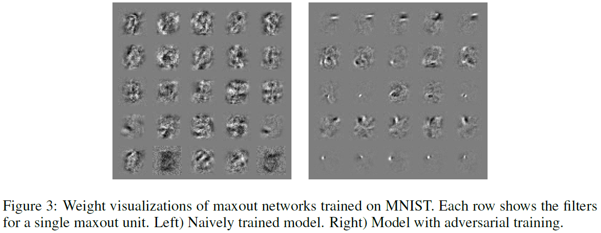
The adversarial example generation can also be used to train neural networks to be more robust against such attacks. For instance, the fast gradient sign method can be used as a regularizer in the training in the following way:

\[J(x, y_{true}) = \alpha J(x, y_{true}) + (1 - \alpha)J(x + \epsilon \cdot sign(\nabla_{x}J(x, y_{true})), y_{true})\]

1.2 Black box models.

Methods in this class have access only to the output of the model.

1.2.1. Pixel attack.

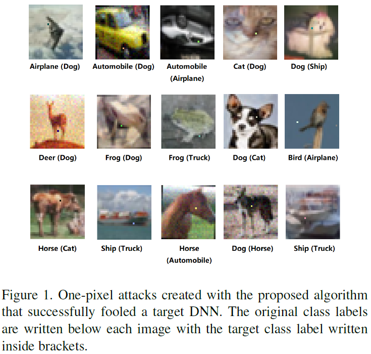
In this approach the attack is extremely limited to the scenario where only one pixel can be modified. The method does not have access to the model or its gradients and it uses the differential evolution method. It requires less adversarial information and can fool more types of networks. The results show that 70.97% of the natural images can be perturbed to at least one target class by modifying just one pixel with 97.47% confidence on average. Thus, the proposed attack explores a different take on adversarial machine learning in an extreme limited scenario, showing that current DNNs are also vulnerable to such low dimension attacks. The problem is formulated as follows: \[max_{e_{x}} f_{y_{fool}}(x + e_{x})\] subject to \(\lVert e_{x}\rVert_{0} \leq d\)

where \(d\) is a small number and the zero norm is defined by the number of non-zero elements in its arguments.

The optimization is carried out using differential evolution algorithm.

2. Generation of noise-like data to fool classifiers.

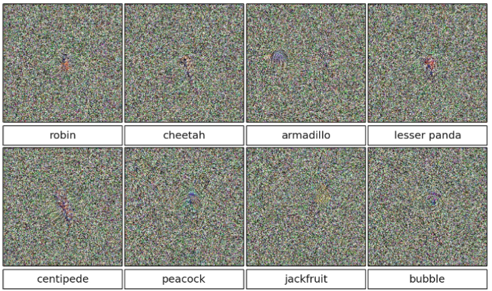
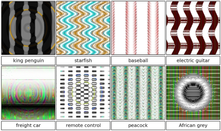
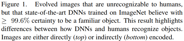
The article by Nguyen et al. [ref: Nguyen et al: Deep Neural Networks are Easily Fooled: High Confidence Predictions for Unrecognizable Images, 2015] showed a method to generate images unrecognizable for human-eyes but state-of-the-art DNNs recognizes these images with high confidence. Their approach is a black-box one. Examples: Irregular noise images

Regular noise images:

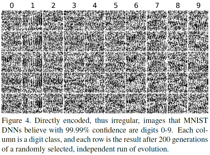
Irregular noise image generation for MNIST digit classification: Here the population consists of a set of images, 28x28 pixels for the MNIST data. Each pixel value is initialized with uniform random noise within the [0, 255] range. Those numbers are independently mutated; first by determining which numbers are mutated, via a rate that starts at 0.1 (each number has a 10% chance of being chosen to be mutated) and drops by half every 1000 generations. The numbers chosen to be mutated are then altered via the polynomial mutation operator with a fixed mutation strength of 15. The recognition ANN network was LeNet to recognize digits from 0 to 9. Therefore the fitness function to be optimized was the model prediction by the LeNet model. Multiple, independent runs of evolution repeatedly produce images that LeNET believes with 99.99% confidence to be digits, but are unrecognizable as such (Fig. 4). In less than 50 generations, each run of evolution repeatedly produces unrecognizable images of each digit type classified by MNIST DNNs with ≥99.99% confidence. By 200 generations, median confidence is 99.99%. Given the DNN’s near certainty, one might expect these images to resemble handwritten digits. On the contrary, the generated images look nothing like the handwritten digits in the MNIST dataset.

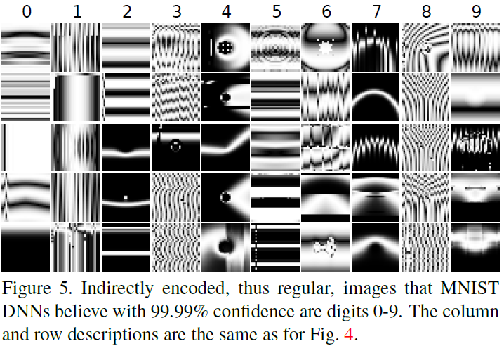
Regular noise image generation for MNIST digit classification: To generate regular noise images, the CPPN was used. CPPNs start with no hidden nodes, and nodes are added over time, encouraging evolution to first search for simple, regular images before adding complexity. The evolved images for class ‘1’ for instance tend to have more vertical bars, while images classified as a 2 tend to have a horizontal bar in the lower half of the image. Qualitatively similar discriminative features are observed in 50 other runs as well (supplementary material). This result suggests that the EA exploits specific discriminative features corresponding to the handwritten digits learned by MNIST DNNs.